Taxa Plot

So, we have tried. From SILVA NGS, RDP Pipeline, MG-RAST to MEGA, and MEGAN...6. 

Two made the cut with my data so far; MEGAN and R.  As a note, I would say the data choose the analysis software.

R yet again gave a beautiful taxa plot. 

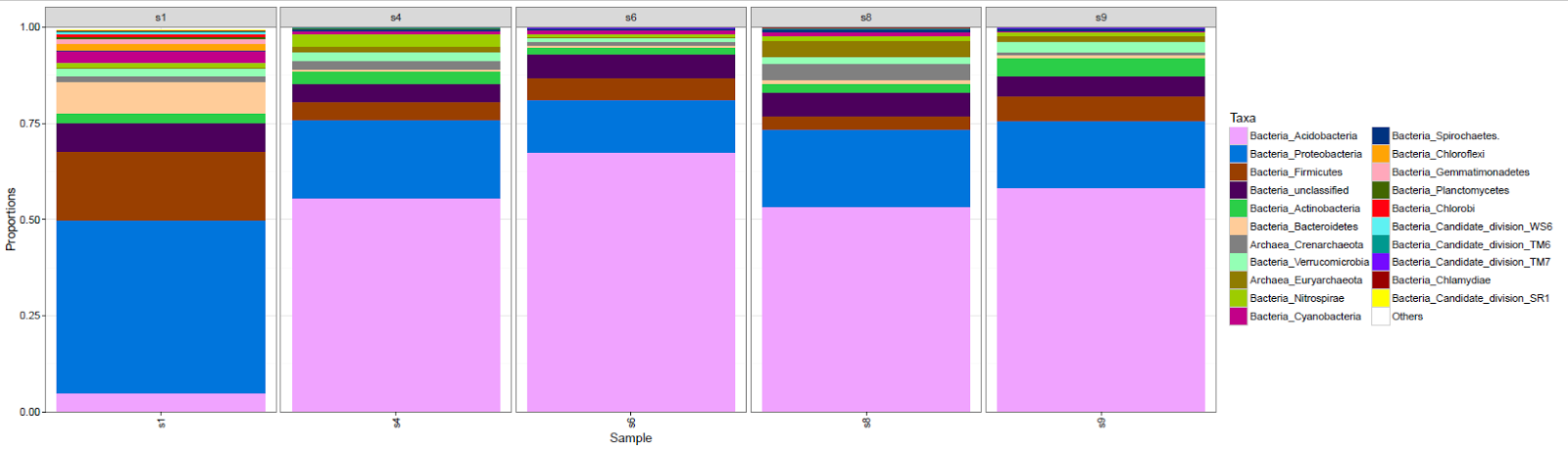
abund_table<-read.csv("SPE_pitlatrine.csv",row.names=1,check.names=FALSE)
 
#Transpose the data to have sample names on rows
abund_table<-t(abund_table)
meta_table<-read.csv("ENV_pitlatrine.csv",row.names=1,check.names=FALSE)
 
#Just a check to ensure that the samples in meta_table are in the same order as in abund_table
meta_table<-meta_table[rownames(abund_table),]
 
#Get grouping information
grouping_info<-data.frame(row.names=rownames(abund_table),t(as.data.frame(strsplit(rownames(abund_table),"_"))))
# > head(grouping_info)
# X1 X2 X3
# T_2_1   T  2  1
# T_2_10  T  2 10
# T_2_12  T  2 12
# T_2_2   T  2  2
# T_2_3   T  2  3
# T_2_6   T  2  6
 
#Apply proportion normalisation
x<-abund_table/rowSums(abund_table)
x<-x[,order(colSums(x),decreasing=TRUE)]
 
#Extract list of top N Taxa
N<-21
taxa_list<-colnames(x)[1:N]
#remove "__Unknown__" and add it to others
taxa_list<-taxa_list[!grepl("Unknown",taxa_list)]
N<-length(taxa_list)
 
#Generate a new table with everything added to Others
new_x<-data.frame(x[,colnames(x) %in% taxa_list],Others=rowSums(x[,!colnames(x) %in% taxa_list]))
 
 
#You can change the Type=grouping_info[,1] should you desire any other grouping of panels
df<-NULL
for (i in 1:dim(new_x)[2]){
  tmp<-data.frame(row.names=NULL,Sample=rownames(new_x),Taxa=rep(colnames(new_x)[i],dim(new_x)[1]),Value=new_x[,i],Type=grouping_info[,1])
  if(i==1){df<-tmp} else {df<-rbind(df,tmp)}
}
colours <- c("#F0A3FF", "#0075DC", "#993F00","#4C005C","#2BCE48","#FFCC99","#808080","#94FFB5","#8F7C00","#9DCC00","#C20088","#003380","#FFA405","#FFA8BB","#426600","#FF0010","#5EF1F2","#00998F","#740AFF","#990000","#FFFF00");
 
 
library(ggplot2)
p<-ggplot(df,aes(Sample,Value,fill=Taxa))+geom_bar(stat="identity")+facet_grid(. ~ Type, drop=TRUE,scale="free",space="free_x")
p<-p+scale_fill_manual(values=colours[1:(N+1)])
p<-p+theme_bw()+ylab("Proportions")
p<-p+ scale_y_continuous(expand = c(0,0))+theme(strip.background = element_rect(fill="gray85"))+theme(panel.margin = unit(0.3, "lines"))
p<-p+theme(axis.text.x=element_text(angle=90,hjust=1,vjust=0.5))
pdf("TAXAplot.pdf",height=6,width=21)
print(p)
dev.off()

Thanks to this website!

http://userweb.eng.gla.ac.uk/umer.ijaz/bioinformatics/ecological.html